Stochastic Gradient Descent with Tensorflow and Keras Framework

Stochastic Gradient Descent(SGD) เป็นวิธีการที่ทำให้ค่า Loss Value ลงไปยังจุดต่ำสุด ซึ่งเมื่อนำไปใช้กับการ Train Model จะส่งผลให้การทำ Deep Learning มีประสิทธิภาพมากยิ่งขึ้น
Gradient Descent Algorithm
Gradient descent เป็นอัลกอรึทึมที่อัพเดพค่า Weight และ Bias วนซ้ำไปเรื่อยๆ เพื่อลด Cost function ให้น้อยที่สุด จากการคำนวณ Gradient(ความชัน) ณ จุดที่เราอยู่แล้วพยายามเดินไปทางตรงข้ามกับ ความชัน ถ้านึกภาพเวลาเราเดินขึ้นภูเขา วิธีการเดินไปให้ถึงจุดสูงสุดคือเราไต่ขึ้นทางที่ชันขึ้นเพื่อไปถึงจุดสูงสุด
Linear Regression with Tensorflow
เริ่มด้วยการเปิด jupyter notebook จะเข้ามาหน้า home ของ jupyter และ New Python3 ขึ้นมาและImport Library ที่จำเป็นเข้ามา

จากนั้นกำหนด Random Seed และจำนวน Epoch ที่จะ Train พร้อมกับ Load ไฟล์ Dataset ชื่อ Real estate.csv
np.random.seed(seed=13)
EPOCH = 500dataset = pd.read_csv('Real estate.csv')
dataset.shape
dataset.describe()


จะใช้ X2 house age มาทำเป็น Input Data หรือตัวแปรอิสระ (Predictor) และ X5 latitude มาทำเป็นผลเฉลย หรือตัวแปรตาม (Response)
Plot X2 house age และ X5 latitude เพื่อดูลักษณะของข้อมูล
dataset.plot(x='X2 house age', y='X5 latitude', style='o')
plt.title('X2 house age vs X5 latitude')
plt.xlabel('X2 house age')
plt.ylabel('X5 latitude')
plt.savefig('X2_X5.jpeg', dpi=300)
plt.show()
ดูการกระจายตัวของ X5 latitude
plt.figure(figsize=(15,10))
plt.tight_layout()
seabornInstance.distplot(dataset['X5 latitude'])
plt.savefig('dis_Width.jpeg', dpi=300)
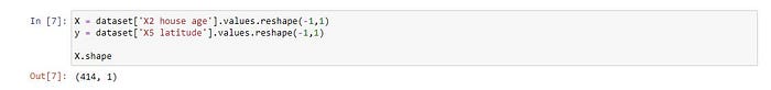
แยก Dataset เป็น Input Data (x) และผลเฉลย (y)
X = dataset['X2 house age'].values.reshape(-1,1)
y = dataset['X5 latitude'].values.reshape(-1,1)X.shape
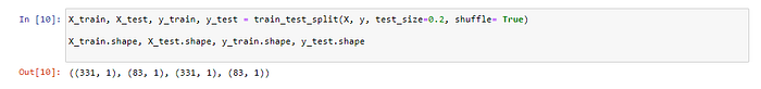
สุ่มแบ่งข้อมูลเป็น 2 ชุด สำหรับ Train 80% และ Test 20%
X_train, X_test, y_train, y_test = train_test_split(X, y, test_size=0.2, shuffle= True)X_train.shape, X_test.shape, y_train.shape, y_test.shape
นิยาม Model ด้วย Tensorflow โดยจะมีการนำ X_train เข้า Model ทั้งก้อนขนาด 331 Row
W = tf.Variable(tf.random.uniform([1], -1.0, 1.0))
b = tf.Variable(tf.random.uniform([1], -1.0, 1.0))y = W * X_train + b

นิยาม Loss Function แบบ Mean Squared Error (MSE)
loss = tf.reduce_mean(tf.square(y - y_train))
กำหนด Optimizer และ Learning Rate
Optimization คือ การหาจุดที่เหมาะสมที่สุด (Optimal Point) จะทำการเปลี่ยนแปลงค่า Weight และค่า Bias โดย Optimizer จะมีการทำ Back-propagation Algorithm เพื่อปรับค่า Weight (W) และ Bias (b) ให้อัตโนมัติ โดยไม่ต้องมีการหาอนุพันธ์ด้วยตัวเอง
optimizer = tf.train.GradientDescentOptimizer(0.0001)train = optimizer.minimize(loss)

เคลียร์ Tensorflow Variable
init = tf.global_variables_initializer()
สร้าง session และรัน init เพื่อเคลียร์ค่า Variable จริงๆ
sess = tf.Session()
sess.run(init)
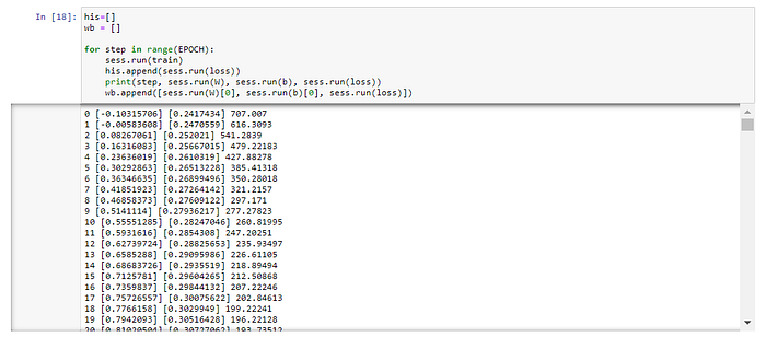
Train Model (sess.run(train))
his=[]
wb = []for step in range(EPOCH):
    sess.run(train)
    his.append(sess.run(loss))
    print(step, sess.run(W), sess.run(b), sess.run(loss))
    wb.append([sess.run(W)[0], sess.run(b)[0], sess.run(loss)])
ดึง Weight (W) และ Bias (b) มาสร้าง Linear Regression Model
M = sess.run(W)
C = sess.run(b)
นิยาม Function Predict
def predict(X, M, C):
    y = M*X+C
    return y[0]
แปลง Loss Value List เป็น DataFrame
df = pd.DataFrame(his, columns=['loss'])
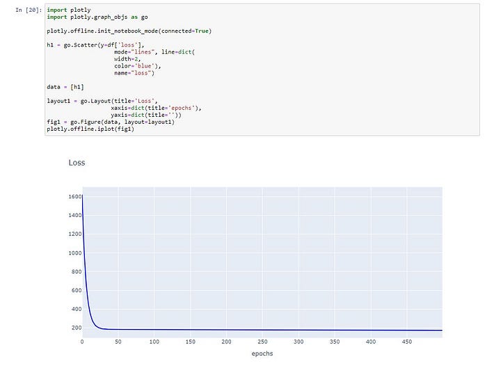
Plot Loss
import plotly
import plotly.graph_objs as goplotly.offline.init_notebook_mode(connected=True)h1 = go.Scatter(y=df['loss'],
                    mode="lines", line=dict(
                    width=2,
                    color='blue'),
                    name="loss")data = [h1]layout1 = go.Layout(title='Loss',
                   xaxis=dict(title='epochs'),
                   yaxis=dict(title=''))
fig1 = go.Figure(data, layout=layout1)
plotly.offline.iplot(fig1)
Predict “X5 latitude”
y_pred = [predict(i, M, C) for i in X_test]y_test.shape

y_test = y_test.reshape(-1)
y_test.shape
แสดงผลการ Predict 10 แถวแรก
df = pd.DataFrame({'Actual': y_test, 'Predicted': y_pred})
df.head(10)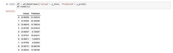
Plot กราฟเปรียบเทียบผลการทำนายกับค่าจริง
df1 = df.head(25)
df1.plot(kind='bar',figsize=(16,10))
plt.grid(which='major', linestyle='-', linewidth='0.5', color='green')
plt.grid(which='minor', linestyle=':', linewidth='0.5', color='black')
plt.show()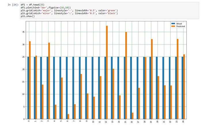
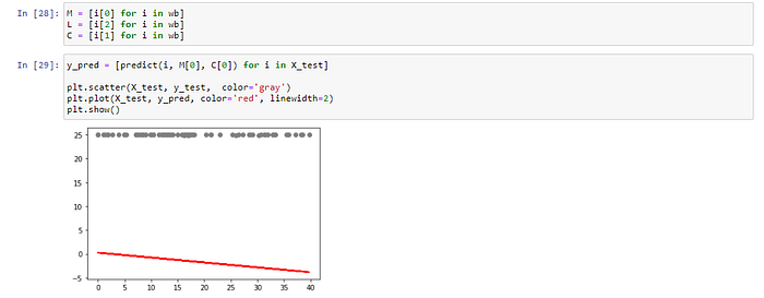
แสดง Model ที่สร้างจากการ Train ใน Epoch ที่ 1
M = [i[0] for i in wb]
L = [i[2] for i in wb]
C = [i[1] for i in wb]y_pred = [predict(i, M[0], C[0]) for i in X_test]plt.scatter(X_test, y_test,  color='gray')
plt.plot(X_test, y_pred, color='red', linewidth=2)
plt.show()
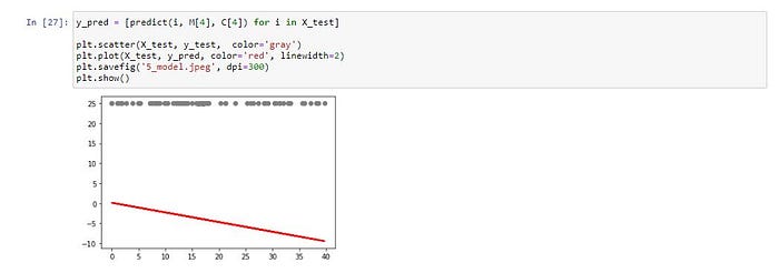
แสดง Model ที่สร้างจากการ Train ใน Epoch ที่ 5
y_pred = [predict(i, M[4], C[4]) for i in X_test]plt.scatter(X_test, y_test,  color='gray')
plt.plot(X_test, y_pred, color='red', linewidth=2)
plt.savefig('5_model.jpeg', dpi=300)
plt.show()
แสดง Model ที่สร้างจากการ Train ใน Epoch ที่ 10
y_pred = [predict(i, M[9], C[9]) for i in X_test]plt.scatter(X_test, y_test,  color='gray')
plt.plot(X_test, y_pred, color='red', linewidth=2)
plt.savefig('10_model.jpeg', dpi=300)
plt.show()

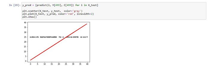
แสดง Model ที่สร้างจากการ Train 500 Epoch
y_pred = [predict(i, M[499], C[499]) for i in X_test]plt.scatter(X_test, y_test,  color='gray')
plt.plot(X_test, y_pred, color='red', linewidth=2)
plt.show()
ดู Loss Value เทียบกับค่า Weight
plt.scatter(M, L,  color='gray')
plt.savefig('weight.jpeg', dpi=300)
plt.show()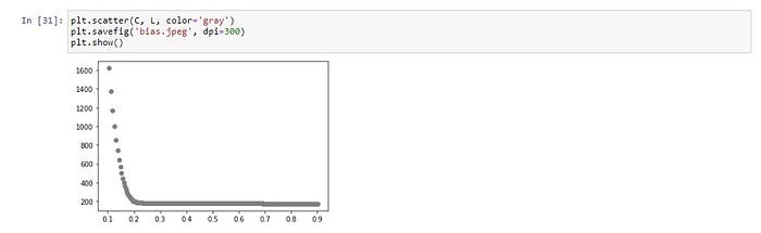
ดู Loss Value เทียบกับค่า Bias
plt.scatter(C, L, color='gray')
plt.savefig('bias.jpeg', dpi=300)
plt.show()
ดู Loss Value เทียบกับค่า Weight และ Bias
import plotly.express as px

df = pd.DataFrame({'W' : M, 'Bias' : C, 'Loss' : L})
fig = px.scatter_3d(df, x='W', y='Bias', z='Loss')
fig.show()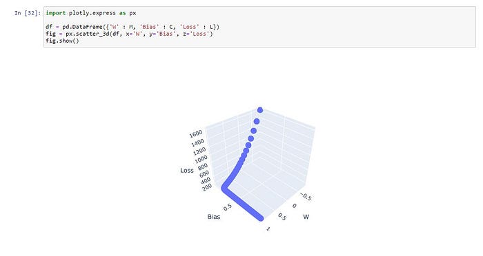
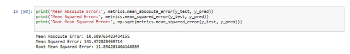
วัดประสิทธิภาพของ Model ด้วย Mean Absolute Error, Mean Squared Error และ Root Mean Squared Error
print('Mean Absolute Error:', metrics.mean_absolute_error(y_test, y_pred))
print('Mean Squared Error:', metrics.mean_squared_error(y_test, y_pred))
print('Root Mean Squared Error:', np.sqrt(metrics.mean_squared_error(y_test, y_pred)))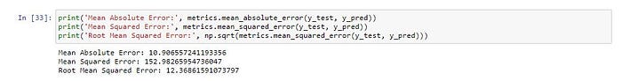
Stochastic Gradient Descent Method Linear Regression with Keras
การสุ่มแบ่ง Dataset เป็นขนาดเล็กๆ (Batch Size) เพื่อนำไป Train Model
Import Library
from tensorflow.python.keras.models import Sequential
from tensorflow.python.keras.layers import Densefrom keras import backend as K
นิยาม Root Mean Squared Error
def rmse(y_true, y_pred):
    return K.sqrt(K.mean(K.square(y_pred - y_true), axis=-1))
นิยาม Model
model = Sequential()
model.add(Dense(1, input_dim=1, kernel_initializer='random_uniform', activation='linear'))
model.summary()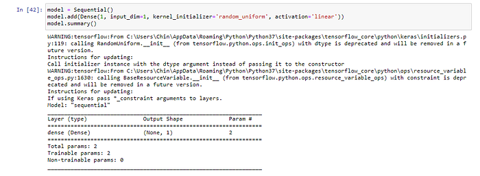
Compile Model
model.compile(loss='mse', optimizer='adam', metrics=['mae', 'mse', rmse])Train Model โดยการสุ่มแบ่งข้อมูลสำหรับ Train 80% และ Validate อีก 20% โดยกำหนด Batch Size เท่ากับ 64
history = model.fit(X_train, y_train, epochs=EPOCH, batch_size=64, verbose=1, validation_split=0.2, shuffle=True)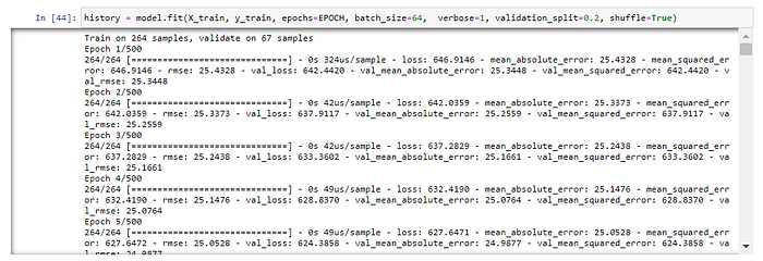
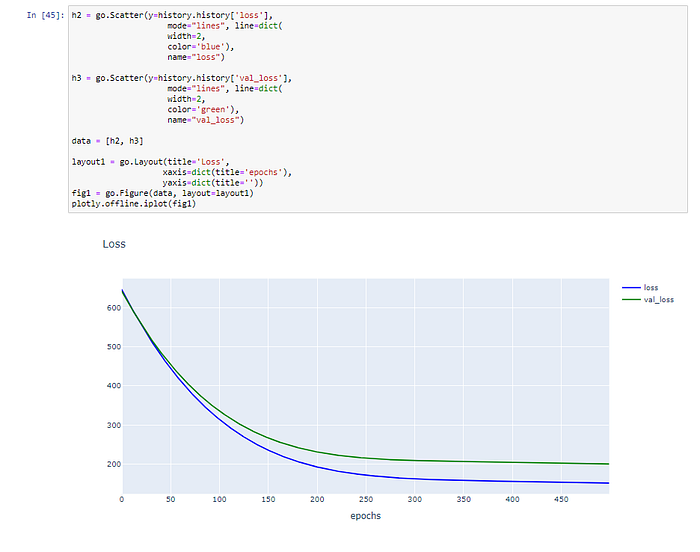
Plot Loss และ Validate Loss
h2 = go.Scatter(y=history.history['loss'],
                    mode="lines", line=dict(
                    width=2,
                    color='blue'),
                    name="loss")h3 = go.Scatter(y=history.history['val_loss'],
                    mode="lines", line=dict(
                    width=2,
                    color='green'),
                    name="val_loss")

data = [h2, h3]layout1 = go.Layout(title='Loss',
                   xaxis=dict(title='epochs'),
                   yaxis=dict(title=''))
fig1 = go.Figure(data, layout=layout1)
plotly.offline.iplot(fig1)
Predict
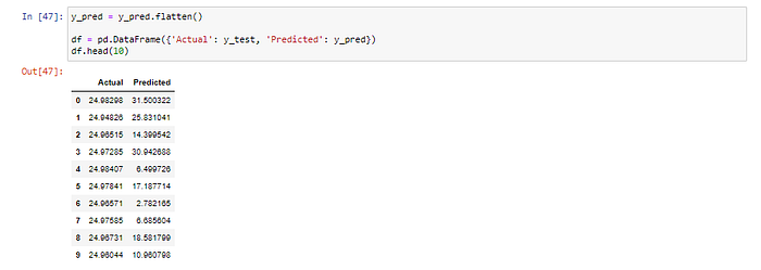
y_pred = model.predict(X_test)แปลงเป็น DataFrame
y_pred = y_pred.flatten()df = pd.DataFrame({'Actual': y_test, 'Predicted': y_pred})
df.head(10)
Plot กราฟเปรียบเทียบผลการทำนายกับค่าจริง
df1 = df.head(25)
df1.plot(kind='bar',figsize=(16,10))
plt.grid(which='major', linestyle='-', linewidth='0.5', color='green')
plt.grid(which='minor', linestyle=':', linewidth='0.5', color='black')
plt.show()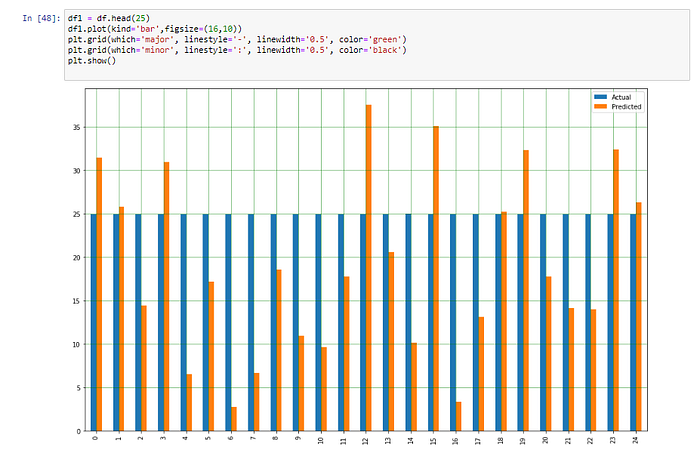
แสดง Model ที่สร้างจากการ Train 500 Epoch
plt.scatter(X_test, y_test,  color='gray')
plt.plot(X_test, y_pred, color='red', linewidth=2)
plt.savefig('keras_500_model.jpeg', dpi=300)
plt.show()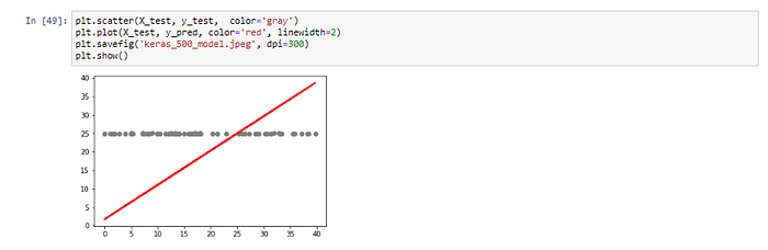
วัดประสิทธิภาพของ Model ด้วย Mean Absolute Error, Mean Squared Error และ Root Mean Squared Error
print('Mean Absolute Error:', metrics.mean_absolute_error(y_test, y_pred))
print('Mean Squared Error:', metrics.mean_squared_error(y_test, y_pred))
print('Root Mean Squared Error:', np.sqrt(metrics.mean_squared_error(y_test, y_pred)))