Feature Engineering for AI and Machine Learning (การทำ Feature Engineering ด้วย Pandas)

Feature Engineering คือ การบวนการใช้ความรู้ Domain Knowledge ในการสร้าง Feature ใหม่ขึ้นมา ตัด Feature ที่ไม่เกี่ยวข้องทิ้งไป เพื่อช่วยทำให้อัลกอริทึมเรียนรู้ได้ดีขึ้น มีวิธีการดังนี้

1. Imputation
2. Handling Outliers
3. Drop Outlier with Standard Deviation
4. Drop with Percentiles
5. Binning
6. Log Transform
7. One-Hot Encoding

ประโยชน์ของการทำ Feature Engineering ก็คือ

• เพื่อเตรียม Dataset ให้พร้อมสำหรับการทำ Data Analytics หรือ เป็น Input ของ Machine Learning Algorithm
• เพื่อเพิ่มประสิทธิภาพให้ Machine Learning Model

Understanding Data Quality

เราจะต้องมีการสำรวจข้อมูลเพื่อพิจารณาคุณภาพของมันในแง่ต่างๆ แล้วจึงเลือกเทคนิคในการทำ Feature Engineering ที่เหมาะสมและต้องมีการนำเข้า library ของ pandas ก่อนเพื่อเข้าใจคุณลักษณะของข้อมูลได้อย่างรวดเร็ว โดยคำนวณมาจากค่าสถิติต่างๆ ด้วย ProfileReport Function และoutput ที่เข้าใจง่าย

ขั้นตอนแรกทำการติดตั้ง Pandas Profiling Library

pip install pandas-profiling[notebook]

จากนั้นเตรียม Dataset และเรียกใช้ ProfileReport Function บน Jupyter Notebook

import numpy as np
import pandas as pd
from pandas_profiling import ProfileReport
df = pd.read_csv("titanic.csv")
profile = ProfileReport(df, title="Pandas Profiling Report")
profile

เราเห็นค่าที่หายไป (Missing Values) ถึง 691 Cell หลังจากนั้นเราจะใช้ Function isnull() และ sum() คำนวนจำนวน (Missing Value ในแต่ละ Column)

print(df.isnull().sum())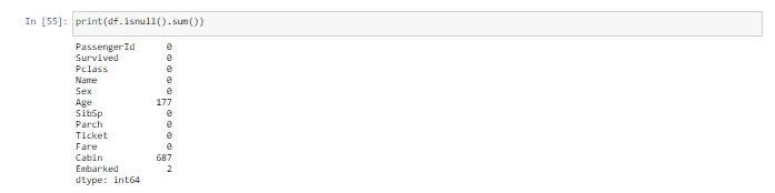

เราสามารถดูข้อมูล 5 แถวแรกได้จากคำสั่ง Function head()

df.head()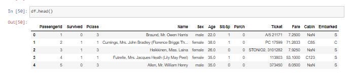

Imputation

จากคำสั่ง df.isnull().sum() เราพบ Column Age เป็น Missing Values ถึง 177 Cell ซึ่งเราจะทดลองแทนที่ Missing Value เหล่านั้นด้วยค่าเฉลี่ยของอายุ ทั้งหมด ใน Column Age โดยใช้ Function fillna()

new_df = df.copy()
new_df['Age'].fillna(df['Age'].mean(), inplace = True)
print(new_df.isnull().sum())

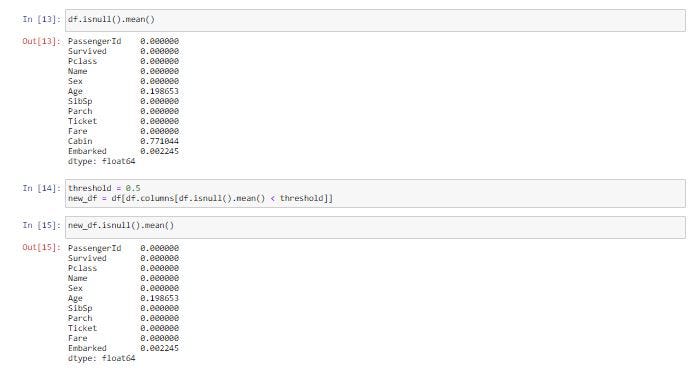
Missing Values ของ Column Age ถูกแทนที่ด้วยค่าเฉลี่ย จึงทำให้พบจำนวน Missing Value เป็น 0 ในบางกรณีการแทนที่ Missing Value ด้วยค่า Mean ก็อาจจะทำให้ได้ข้อมูลที่ไม่ตรงกับที่ต้องการ ซึ่งเราอาจจะใช้การลบ Row หรือ Column ทิ้งจากการกำหนดค่า Threshold ดังตัวอย่างด้านล่าง จะทำให้ Column ที่มีร้อยละของ Missing Value มากกว่า 50% คือ Column Cabin ถูกลบ

df.isnull().mean()
threshold = 0.5
new_df = df[df.columns[df.isnull().mean() < threshold]]
new_df.isnull().mean()

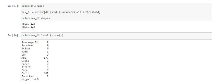
ขณะที่การลบ Row ที่มีร้อยละของ Missing Value มากกว่า 50% จะใช้คำสั่ง

print(df.shape)
new_df = df.loc[df.isnull().mean(axis=1) < threshold]
print(new_df.shape)

print(new_df.isnull().sum())

ว่าจำนวน Row จะลดลงไปเท่าไร

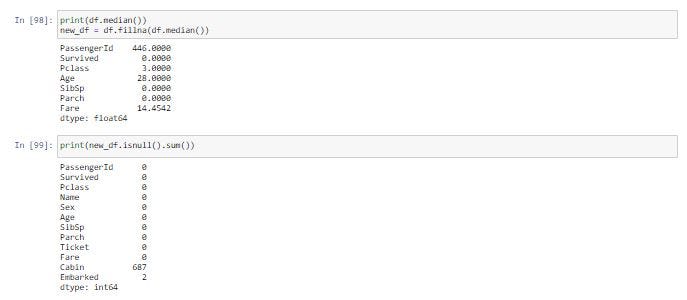
ค่ามัธยฐานของแต่ละ Column แทน เนื่องจากค่ามัธยฐานมีความทนทานต่อ Outlier Value ได้มากกว่า “ค่า outlier value คือ ค่าเฉลี่ยของคอลัมบ์มีความ sensitive”ดังตัวอย่างต่อไปนี้

print(df.median())
new_df = df.fillna(df.median())
print(new_df.isnull().sum())

ถ้าอยากให้ Missing Value ทุก Cell ด้วย 0 จะใช้คำสั่งต่อไปนี้

new_df = df.fillna(0)
print(new_df.isnull().sum())

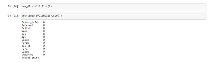
แต่การแทน Missing Value ด้วย 0 จะทำให้ Cell ที่มีชนิดข้อมูลแบบ String เป็น 0 ด้วยเช่นกัน ดังเช่นใน Cell ของ Column Cabin ซึ่งเป็นสิ่งที่เราไม่ต้องการ

อีกวิธีหนึ่งคือการลบทั้งแถวทิ้ง ในกรณีที่พบ Cell หนึ่ง Cell ใดมี Missing Value ซึ่งจะเป็นวิธีการที่ดีถ้าไม่ทำให้มีข้อมูลหายไปเป็นจำนวนมาก

print(df.shape)
new_df = df.dropna(how='any')
print(new_df.shape)

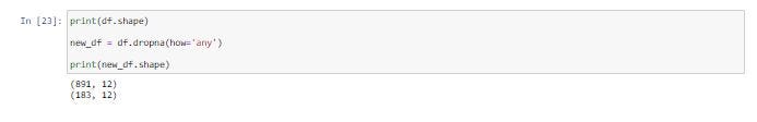
พบว่ามีข้อมูลถูกลบไปมากกว่า 708 Row

Handling Outliers

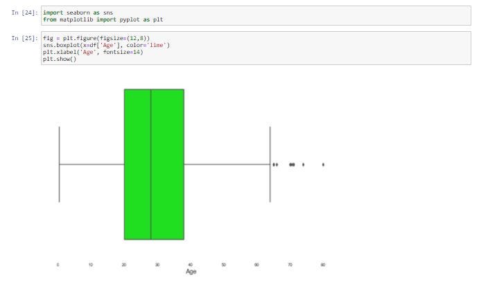
Outlier หรือค่าที่ผิดปกติ คือ ข้อมูลที่มีค่าสูง หรือต่ำกว่าข้อมูลส่วนใหญ่ในชุดข้อมูลหนึ่งๆ อย่างมาก การจัดการกับ Outlier จะพิจารณาจาก Standard Deviation และ Percentile เราจะทำ Data Visualization เพื่อดูลักษณะการกระจายของข้อมูล และ Outlier จาก Function boxplot() ของ Seaborn Library

import seaborn as sns
from matplotlib import pyplot as plt
fig = plt.figure(figsize=(12,8))
sns.boxplot(x=df['Age'], color='lime')
plt.xlabel('Age', fontsize=14)
plt.show()

df['Age'].describe()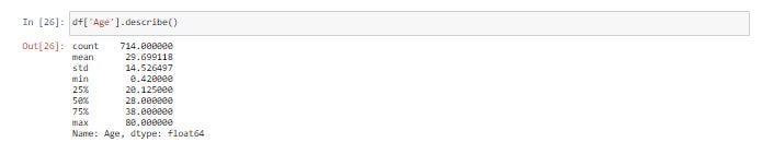

จากภาพเป็นการแสดงลักษณะการกระจายของข้อมูล และ Outlier ของ Column age ซึ่งพบอายุที่สูงกว่าข้อมูลส่วนใหญ่ (Outlier) ทางด้านขวามือของภาพ โดยอายุมีค่าเฉลี่ยที่ 29.6 ปีแต่มีอายุสูงสุด 80 ปี

Drop Outlier with Standard Deviation

ซึ่งเมื่อดูลักษณะการกระจายของข้อมูล และ Outlier จะพบว่าค่าเฉลี่ยของอายุจะลดลงมาที่ 29.5 ปีและอายุสูงสูงอยู่ที่ 71 ปี

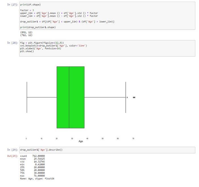
print(df.shape)
factor = 3
upper_lim = df['Age'].mean () + df['Age'].std () * factor
lower_lim = df['Age'].mean () - df['Age'].std () * factor
drop_outlier1 = df[(df['Age'] < upper_lim) & (df['Age'] > lower_lim)]
print(drop_outlier1.shape)
fig = plt.figure(figsize=(12,8))
sns.boxplot(x=drop_outlier1['Age'], color='lime')
plt.xlabel('Age', fontsize=14)
plt.show()
drop_outlier1['Age'].describe()

Drop with Percentiles

นอกจากนี้เราสามารถลบแถวที่พบ Outlier ใน Column price ที่น้อยกว่าหรือเท่ากับ Quantile 0.5 และมากกว่าหรือเท่ากับ Quantile 0.95 ตามภาพข้างล่าง

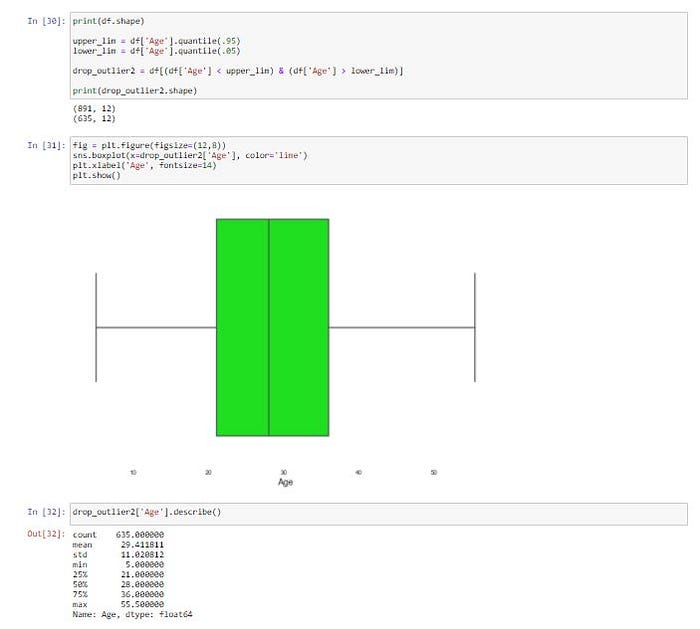
print(df.shape)
upper_lim = df['Age'].quantile(.95)
lower_lim = df['Age'].quantile(.05)
drop_outlier2 = df[(df['Age'] < upper_lim) & (df['Age'] > lower_lim)]
print(drop_outlier2.shape)
fig = plt.figure(figsize=(12,8))
sns.boxplot(x=drop_outlier2['Age'], color='lime')
plt.xlabel('Age', fontsize=14)
plt.show()
drop_outlier2.sample(n=5).head()

Binning

การทำ Binning หรือการแบ่งข้อมูลออกตามช่วงที่กำหนด จะทำให้สามารถป้องกันการเกิด Overfitting เมื่อมีการ Train Model ได้ในระดับหนึ่ง

labels = ['low', 'mid', 'high']
bins = [0., 20., 40., 100.]
drop_outlier2['Age'] = pd.cut(drop_outlier2['Age'], labels=labels, bins=bins, include_lowest=False)

drop_outlier2.sample(n=5).head()

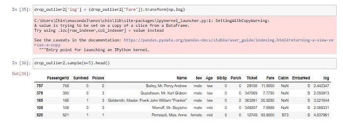
Log Transform

Log Transform เป็นการใช้ Log ทางคณิตศาสตร์แปลงข้อมูล ซึ่งจะช่วยลดการเบ้ของข้อมูล โดยหลังการแปลงข้อมูลแล้ว จะทำให้การกระจายตัวเข้าสู่ Normal Distribution มากขึ้น

drop_outlier2['log'] = (drop_outlier2['Fare']).transform(np.log)
drop_outlier2.sample(n=5).head()

One-hot Encoding

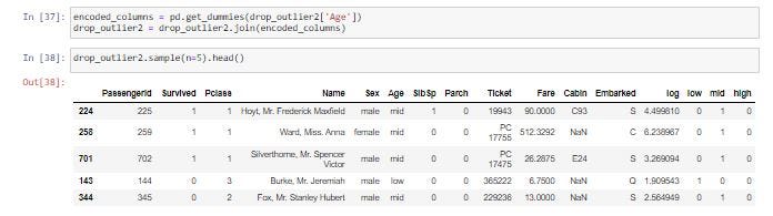
One-hot Encoding เป็นการเข้ารหัสข้อมูลแบบหนึ่งที่มักจะใช้กันบ่อยในงานทางด้าน Machine Learning โดยการขยายข้อมูลจากเดิมที่มี Column เดียว เป็นค่า 0 และ 1 หลายๆ Column ตามจำนวนหมวดหมู่ของข้อมูลใน Column เดิม โดยจะมีการกำหนดค่าเป็น 1 ใน Column ใหม่ และตำแหน่งของ Column จะแทนลำดับของหมวดหมู่ของข้อมูลเดิม แล้วกำหนดค่า 0 ใน Column อื่นๆ ที่เหลือ

encoded_columns = pd.get_dummies(drop_outlier2['Age'])
drop_outlier2 = drop_outlier2.join(encoded_columns)
drop_outlier2.sample(n=5).head()

จบการนำเสนอขอบคุณครับ…